Transforming data
You can transform and manipulate data using many different techniques in Data load editor.
One of the advantages to data manipulation is that you can choose to load only a subset of the data from a file, such as a few chosen columns from a table, to make the data handling more efficient. You can also load the data more than once to split up the raw data into several new logical tables. It is also possible to load data from more than one source and merge it into one table in Qlik Sense.
In this topic, you will perform some basic data transformation using a Resident load, and then a Preceding load.
Resident LOAD
You can use the Resident source qualifier in a LOAD statement to load data from a previously loaded table. This is also useful when you want to perform calculations on data loaded with a SELECT statement where you do not have the option to use Qlik Sense functions, such as date or numeric value handling.
In this example, you will create a new table called Sales_Buckets and then load the data from Table1 using a resident load. In the Sales_Buckets table, you will create a variable called quantity_threshold, and then use a Where statement to only load data that meets that threshold.
- Open the Data load editor in the Scripting Tutorial app.
- Click the Sales tab.
- Add the following to the end of your script:
- Click Load data.
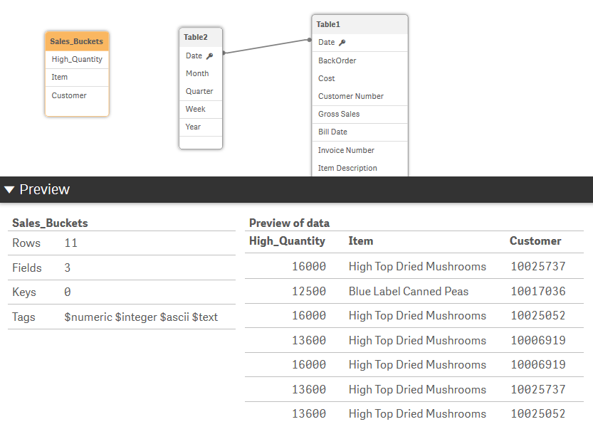
- Open the Data model viewer. You can see that you created a new table called Sales_Buckets with the data loaded according to the fields that you specified, and the threshold that you set.
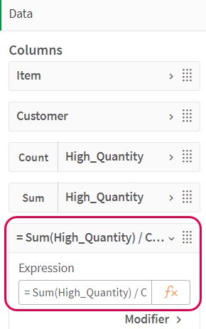
- Add the data to a table in your app. Add Item and Customer as dimensions. Add High-Quantity as a measure aggregated on Count, and then again aggregated on Sum. Next, add a new column as a measure with the following formula:
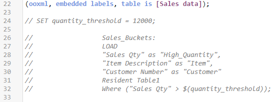
- Now that we have completed this example, comment out the script for the quantity_threshold variable and the Sales_Buckets table.
SET quantity_threshold = 12000;

					Sales_Buckets:
					LOAD
					"Sales Qty" as "High_Quantity",
					"Item Description" as "Item",
					"Customer Number" as "Customer"
					Resident Table1
					Where ("Sales Qty" > $(quantity_threshold));
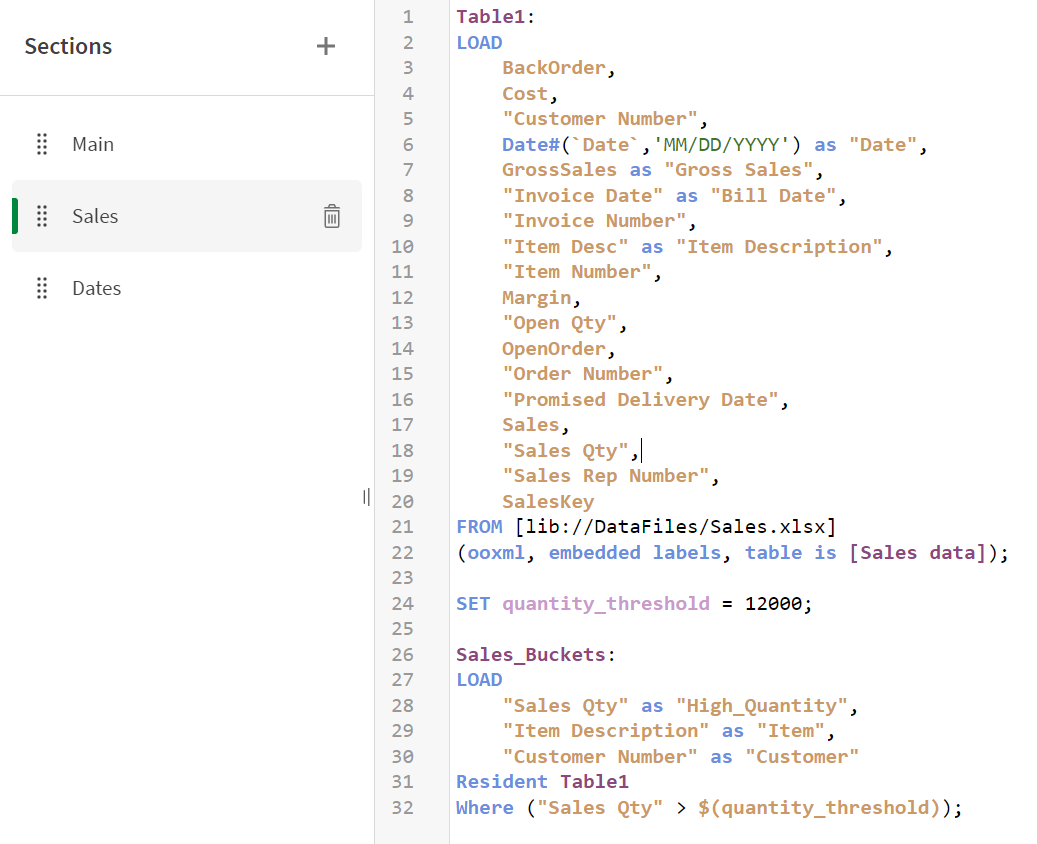
Your script should look like this:
Load script window with script to create new table called Sales_Buckets
Sales_Buckets table in data model viewer
= Sum(High_Quantity) / Count(High_Quantity)New measure with formula
Your table shows, for example, that Customer 10025737 has made 4 large orders of High Top Dried Mushrooms, with an average quantity of 14,800. To perform sorts on the data in the fields, close Edit mode by clicking Done.
Table showing customers that have made large orders

The end of your script should now appear as follows:
Commented out script
Preceding LOAD
A preceding load allows you to perform transformations and apply filters so that you can load data in one pass. Basically, it is a LOAD statement that loads from the LOAD or SELECT statement below, without specifying a source qualifier such as From or Resident that you would normally do. You can stack any number of LOAD statements this way. The statement at the bottom will be evaluated first, then the statement above that, and so on until the top statement has been evaluated.
As mentioned earlier in this tutorial, you can load data into Qlik Sense using the LOAD and SELECT statements. Each of these statements generates an internal table. LOAD is used to load data from files or from an inline table, while SELECT is used to load data from databases. You have used data from files in this tutorial. In this example, you will use an inline table. However, it is worth noting that a preceding load can be used above a SELECT statement to manipulate your data. The basics are the same as you will see here using LOAD.
This example is not related to the data we are loading in this tutorial. It is only used to show an example of what a preceding load can look like. You will create an inline table in the data load editor called Transactions. Date interpretation will be performed in the preceding LOAD, where a new field called transaction_date will be created. This field is created from the sale_date field.
- Create a new app and call it ReformatDate.
- Open the data load editor, and then create a new tab called TransactionData.
- Add the following script:
- Click Load data.
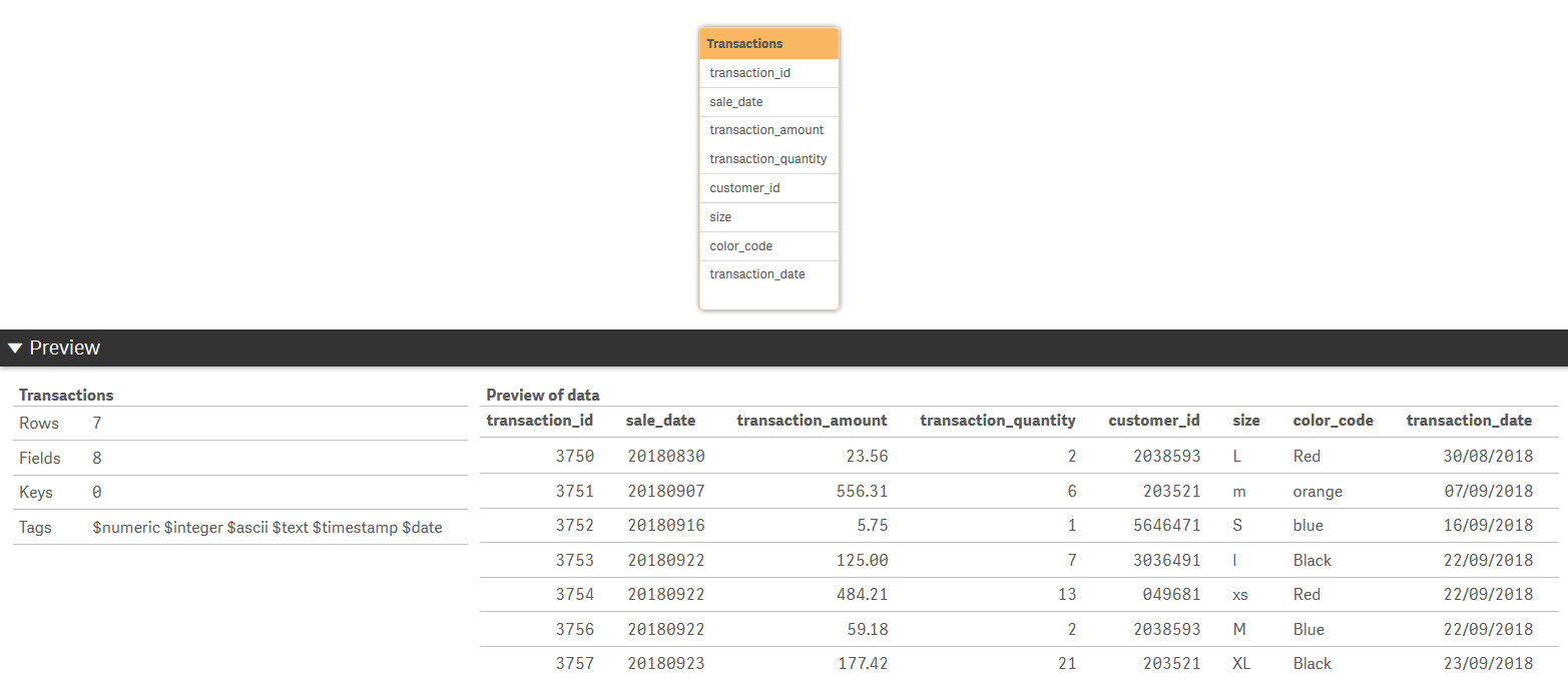
- Open the Data model viewer. Select and expand the Transactions table. You can see that all the fields were loaded as specified by the * in the preceding load statement. A new field called transaction_date was created. The field has the reformatted date.
Transactions:
Load *,
Date(Date#(sale_date,'YYYYMMDD'),'DD/MM/YYYY') as transaction_date;
Load * Inline [ transaction_id, sale_date, transaction_amount, transaction_quantity, customer_id, size, color_code
3750, 20180830, 23.56, 2, 2038593, L, Red
3751, 20180907, 556.31, 6, 203521, m, orange
3752, 20180916, 5.75, 1, 5646471, S, blue
3753, 20180922, 125.00, 7, 3036491, l, Black
3754, 20180922, 484.21, 13, 049681, xs, Red
3756, 20180922, 59.18, 2, 2038593, M, Blue
3757, 20180923, 177.42, 21, 203521, XL, Black ];
Your script should look like this:
Load script with preceding load

New field called transaction_date in data model viewer
